
Smart grid model with renewable energy sources in MATLAB Simulink
Introduction to Smart Grids
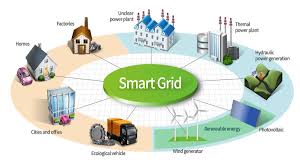
Smart grids represent the future of electrical power distribution, combining traditional power infrastructure with advanced digital communication technologies. Unlike conventional power grids, smart grids can automatically detect and respond to local changes in usage, integrate renewable energy sources efficiently, and provide real-time information to both utilities and consumers.
In this comprehensive tutorial, we'll explore smart grid concepts through practical MATLAB Simulink simulation, covering:
- Bidirectional power flow management
- Renewable energy integration (Solar & Wind)
- Energy storage systems (Battery & Supercapacitors)
- Load balancing and demand response
- Grid stability and protection systems
Prerequisites
Basic knowledge of electrical circuits, power systems fundamentals, and familiarity with MATLAB/Simulink interface. Understanding of AC power analysis and three-phase systems is recommended.
Smart Grid Components
Before diving into simulation, let's understand the key components that make a grid "smart":
Setting Up the Simulink Model
We'll build a comprehensive smart grid model step by step. Start by opening MATLAB and creating a new Simulink model:
% MATLAB Commands to initialize the workspace
clear all; clc;

% Define simulation parameters
sim_time = 10; % Simulation time in seconds
solar_capacity = 100e3; % 100 kW solar capacity
wind_capacity = 150e3; % 150 kW wind capacity
battery_capacity = 200e3; % 200 kWh battery capacity
base_load = 180e3; % 180 kW base load

% Grid parameters
grid_voltage = 11e3; % 11 kV distribution voltage
grid_frequency = 50; % 50 Hz
1. Traditional Grid Source
First, let's model the traditional grid connection:
% Grid Source Block Configuration
% Use: Three-Phase Source (Simulink/SimPowerSystems/Electrical Sources)
% Parameters:
% - Peak line-to-line voltage: 11000*sqrt(2) V
% - Frequency: 50 Hz
% - Phase angle: 0 degrees
% - Internal resistance: 0.01 ohm
% - Internal inductance: 1e-6 H
2. Solar Power Generation
Model a solar PV system with MPPT controller:
function [P_solar, V_dc] = solarPVModel(irradiance, temperature)
    % Solar PV model with temperature and irradiance variation

    % Standard conditions
    G_std = 1000; % W/m^2
    T_std = 25; % °C

    % PV module parameters
    V_oc = 40; % Open circuit voltage
    I_sc = 8.5; % Short circuit current
    V_mp = 32; % Voltage at maximum power
    I_mp = 7.8; % Current at maximum power

    % Temperature coefficients
    alpha = 0.0032; % Current temperature coefficient
    beta = -0.0032; % Voltage temperature coefficient

    % Calculate actual values
    I_sc_actual = I_sc * (irradiance/G_std) * (1 + alpha*(temperature-T_std));
    V_oc_actual = V_oc * (1 + beta*(temperature-T_std));

    % Simplified MPPT - assume operating at 80% of Voc
    V_dc = 0.8 * V_oc_actual;
    I_dc = I_sc_actual * 0.9; % Simplified current calculation

    P_solar = V_dc * I_dc;
end
3. Wind Power Generation
Implement a wind turbine model with variable wind speed:
function P_wind = windTurbineModel(wind_speed)
    % Wind turbine power curve

    % Turbine specifications
    P_rated = 150e3; % 150 kW rated power
    v_cut_in = 3; % Cut-in wind speed (m/s)
    v_rated = 12; % Rated wind speed (m/s)
    v_cut_out = 25; % Cut-out wind speed (m/s)

    if wind_speed < v_cut_in || wind_speed > v_cut_out
        P_wind = 0;
    elseif wind_speed < v_rated
        % Cubic relationship in Region 2
        P_wind = P_rated * ((wind_speed - v_cut_in)/(v_rated - v_cut_in))^3;
    else
        % Constant power in Region 3
        P_wind = P_rated;
    end

    % Add turbulence factor
    turbulence = 1 + 0.1*randn(); % 10% turbulence
    P_wind = P_wind * max(0, turbulence);
end
Energy Storage System
Implement a battery energy storage system with state-of-charge management:
function [P_battery, SOC] = batteryModel(P_demand, P_generation, SOC_prev, dt)
    % Battery Energy Storage System model

    % Battery parameters
    capacity = 200e3; % 200 kWh capacity
    efficiency_charge = 0.95;
    efficiency_discharge = 0.95;
    SOC_min = 0.2; % Minimum 20% SOC
    SOC_max = 0.9; % Maximum 90% SOC
    max_charge_power = 100e3; % 100 kW max charging
    max_discharge_power = 100e3; % 100 kW max discharging

    % Calculate power imbalance
    P_imbalance = P_generation - P_demand;

    if P_imbalance > 0 && SOC_prev < SOC_max
        % Excess generation - charge battery
        P_battery = -min(P_imbalance * efficiency_charge, max_charge_power);
        % Update SOC
        energy_change = -P_battery * dt / 3600; % Convert to kWh
        SOC = SOC_prev + energy_change / capacity;
        SOC = min(SOC, SOC_max);

    elseif P_imbalance < 0 && SOC_prev > SOC_min
        % Deficit - discharge battery
        P_battery = min(-P_imbalance / efficiency_discharge, max_discharge_power);
        % Update SOC
        energy_change = P_battery * dt / 3600; % Convert to kWh
        SOC = SOC_prev - energy_change / capacity;
        SOC = max(SOC, SOC_min);

    else
        % No battery action
        P_battery = 0;
        SOC = SOC_prev;
    end
end
Load Modeling and Demand Response
Smart grids enable demand response - the ability to modify consumer demand patterns:
function [P_load, P_critical, P_flexible] = smartLoadModel(t, price_signal)
    % Smart load model with demand response capability

    % Base load profile (typical residential/commercial)
    hour = mod(t/3600, 24); % Convert time to hour of day

    % Typical daily load curve
    if hour >= 0 && hour < 6
        base_factor = 0.6; % Low demand during night
    elseif hour >= 6 && hour < 9
        base_factor = 0.9; % Morning peak
    elseif hour >= 9 && hour < 17
        base_factor = 0.8; % Daytime
    elseif hour >= 17 && hour < 22
        base_factor = 1.0; % Evening peak
    else
        base_factor = 0.7; % Late evening
    end

    % Critical load (cannot be reduced)
    P_critical = 120e3 * base_factor * 0.6; % 60% of load is critical

    % Flexible load (can respond to price signals)
    base_flexible = 120e3 * base_factor * 0.4; % 40% is flexible

    % Demand response based on price
    price_threshold = 0.15; % $/kWh threshold
    if price_signal > price_threshold
        % Reduce flexible load when prices are high
        reduction_factor = min(0.5, (price_signal - price_threshold) * 2);
        P_flexible = base_flexible * (1 - reduction_factor);
    else
        P_flexible = base_flexible;
    end

    P_load = P_critical + P_flexible;
end
Grid Control and Optimization
Implement an energy management system that optimizes power flow:
function control_signals = energyManagementSystem(grid_data)
    % Energy Management System - optimization and control

    % Extract current state
    P_solar = grid_data.solar_power;
    P_wind = grid_data.wind_power;
    P_load = grid_data.load_demand;
    SOC = grid_data.battery_soc;
    grid_price = grid_data.electricity_price;

    % Total renewable generation
    P_renewable = P_solar + P_wind;

    % Initialize control signals
    control_signals.battery_mode = 'standby';
    control_signals.grid_import = 0;
    control_signals.load_shed = 0;

    % Power balance calculation
    P_balance = P_renewable - P_load;

    if P_balance > 50e3 && SOC < 0.9
        % Excess renewable power - charge battery
        control_signals.battery_mode = 'charge';
        control_signals.battery_power = min(P_balance, 100e3);

    elseif P_balance < -20e3 && SOC > 0.3
        % Power deficit - discharge battery
        control_signals.battery_mode = 'discharge';
        control_signals.battery_power = min(-P_balance, 100e3);
        P_balance = P_balance + control_signals.battery_power;

    end

    % Grid interaction
    if P_balance < -10e3
        % Still have deficit - import from grid
        control_signals.grid_import = -P_balance;
    elseif P_balance > 10e3
        % Excess power - export to grid (if allowed)
        control_signals.grid_export = P_balance;
    end

    % Emergency load shedding if needed
    if control_signals.grid_import > 200e3 % Grid import limit
        excess_demand = control_signals.grid_import - 200e3;
        control_signals.load_shed = excess_demand;
        control_signals.grid_import = 200e3;
    end
end
Simulation Results and Analysis
Run the complete simulation and analyze the results:
% Complete simulation script
function runSmartGridSimulation()
    % Simulation parameters
    dt = 0.1; % Time step (seconds)
    t_end = 86400; % 24 hours simulation
    t = 0:dt:t_end;
    n = length(t);

    % Initialize result arrays
    results.time = t;
    results.solar_power = zeros(1, n);
    results.wind_power = zeros(1, n);
    results.load_demand = zeros(1, n);
    results.battery_power = zeros(1, n);
    results.battery_soc = zeros(1, n);
    results.grid_power = zeros(1, n);

    % Initial conditions
    SOC = 0.5; % 50% initial SOC

    % Run simulation
    for i = 1:n
        current_time = t(i);

        % Environmental conditions (varying throughout the day)
        irradiance = 1000 * max(0, sin(pi * current_time / 43200)); % Solar irradiance
        temperature = 25 + 10 * sin(pi * current_time / 43200); % Temperature variation
        wind_speed = 8 + 4 * sin(pi * current_time / 21600) + randn(); % Wind variation

        % Generate power from renewables
        [P_solar, ~] = solarPVModel(irradiance, temperature);
        P_wind = windTurbineModel(wind_speed);

        % Calculate load demand
        electricity_price = 0.1 + 0.05 * sin(pi * current_time / 43200); % Variable pricing
        [P_load, ~, ~] = smartLoadModel(current_time, electricity_price);

        % Battery management
        P_renewable = P_solar + P_wind;
        [P_battery, SOC] = batteryModel(P_load, P_renewable, SOC, dt);

        % Grid power (positive = import, negative = export)
        P_grid = P_load - P_renewable - P_battery;

        % Store results
        results.solar_power(i) = P_solar;
        results.wind_power(i) = P_wind;
        results.load_demand(i) = P_load;
        results.battery_power(i) = P_battery;
        results.battery_soc(i) = SOC;
        results.grid_power(i) = P_grid;
    end

    % Plot results
    plotSmartGridResults(results);
end

function plotSmartGridResults(results)
    figure('Position', [100, 100, 1200, 800]);

    % Power flow subplot
    subplot(2,2,1);
    plot(results.time/3600, results.solar_power/1000, 'y-', 'LineWidth', 2);
    hold on;
    plot(results.time/3600, results.wind_power/1000, 'b-', 'LineWidth', 2);
    plot(results.time/3600, results.load_demand/1000, 'r-', 'LineWidth', 2);
    plot(results.time/3600, results.grid_power/1000, 'k-', 'LineWidth', 2);
    xlabel('Time (hours)');
    ylabel('Power (kW)');
    title('Smart Grid Power Flow');
    legend('Solar', 'Wind', 'Load', 'Grid', 'Location', 'best');
    grid on;

    % Battery status subplot
    subplot(2,2,2);
    yyaxis left;
    plot(results.time/3600, results.battery_power/1000, 'g-', 'LineWidth', 2);
    ylabel('Battery Power (kW)');
    yyaxis right;
    plot(results.time/3600, results.battery_soc*100, 'm-', 'LineWidth', 2);
    ylabel('SOC (%)');
    xlabel('Time (hours)');
    title('Battery Energy Storage System');
    grid on;

    % Energy balance subplot
    subplot(2,2,3);
    renewable_energy = (results.solar_power + results.wind_power)/1000;
    plot(results.time/3600, renewable_energy, 'g-', 'LineWidth', 2);
    hold on;
    plot(results.time/3600, results.load_demand/1000, 'r-', 'LineWidth', 2);
    xlabel('Time (hours)');
    ylabel('Power (kW)');
    title('Renewable vs Load');
    legend('Renewable Generation', 'Load Demand', 'Location', 'best');
    grid on;

    % Grid interaction subplot
    subplot(2,2,4);
    grid_import = max(0, results.grid_power/1000);
    grid_export = max(0, -results.grid_power/1000);
    plot(results.time/3600, grid_import, 'r-', 'LineWidth', 2);
    hold on;
    plot(results.time/3600, grid_export, 'b-', 'LineWidth', 2);
    xlabel('Time (hours)');
    ylabel('Power (kW)');
    title('Grid Interaction');
    legend('Import from Grid', 'Export to Grid', 'Location', 'best');
    grid on;
end
Key Performance Indicators
Monitor renewable energy penetration (%), grid import/export balance, battery utilization, load factor, and power quality metrics to evaluate smart grid performance.
Advanced Features
1. Voltage Regulation
Smart grids must maintain voltage within acceptable limits despite variable generation:
function V_regulated = voltageRegulation(V_measured, P_reactive)
    % Automatic Voltage Regulator for smart grid

    V_reference = 1.0; % Per unit reference voltage
    V_tolerance = 0.05; % ±5% tolerance

    % PI controller parameters
    Kp = 2.0;
    Ki = 0.5;

    persistent integral_error;
    if isempty(integral_error)
        integral_error = 0;
    end

    % Calculate error
    voltage_error = V_reference - V_measured;
    integral_error = integral_error + voltage_error;

    % PI controller output
    Q_correction = Kp * voltage_error + Ki * integral_error;

    % Apply reactive power correction
    P_reactive_new = P_reactive + Q_correction;

    % Simplified voltage calculation
    V_regulated = V_measured + 0.1 * Q_correction;

    % Limit voltage within acceptable range
    V_regulated = max(V_reference - V_tolerance, ...
                     min(V_reference + V_tolerance, V_regulated));
end
2. Fault Detection and Protection
function fault_status = faultDetection(I_measured, V_measured)
    % Smart grid fault detection system

    % Protection settings
    I_threshold = 1.5; % 150% of rated current
    V_threshold_low = 0.8; % 80% of rated voltage
    V_threshold_high = 1.2; % 120% of rated voltage

    fault_status.overcurrent = max(I_measured) > I_threshold;
    fault_status.undervoltage = min(V_measured) < V_threshold_low;
    fault_status.overvoltage = max(V_measured) > V_threshold_high;
    fault_status.any_fault = fault_status.overcurrent || ...
                            fault_status.undervoltage || ...
                            fault_status.overvoltage;

    if fault_status.any_fault
        fprintf('FAULT DETECTED: ');
        if fault_status.overcurrent
            fprintf('Overcurrent ');
        end
        if fault_status.undervoltage
            fprintf('Undervoltage ');
        end
        if fault_status.overvoltage
            fprintf('Overvoltage ');
        end
        fprintf('\n');
    end
end
Simulation Limitations
Remember that these are simplified models for educational purposes. Real smart grid systems involve complex dynamics, detailed power electronics models, and sophisticated control algorithms that require more advanced simulation tools.
Benefits of Smart Grid Technology
| Benefit | Traditional Grid | Smart Grid |
|---|---|---|
| Renewable Integration | Limited, causes instability | High integration with stability |
| Outage Detection | Customer calls required | Automatic detection |
| Energy Efficiency | Fixed consumption patterns | Demand response optimization |
| Power Quality | Basic regulation | Advanced monitoring & control |
Future Developments
The evolution of smart grids continues with emerging technologies:
- Artificial Intelligence: Machine learning for predictive maintenance and optimization
- Blockchain: Peer-to-peer energy trading and secure transactions
- 5G Communication: Ultra-low latency for real-time control
- Edge Computing: Distributed intelligence at grid nodes
- Electric Vehicle Integration: V2G (Vehicle-to-Grid) capabilities
Conclusion
Smart grid simulation using MATLAB Simulink provides invaluable insights into modern power system operation. The integration of renewable energy sources, energy storage, and intelligent control systems creates a more resilient, efficient, and sustainable electrical grid.
This tutorial covered the fundamental aspects of smart grid modeling, from individual component models to system-level optimization. The simulation framework can be extended to explore specific aspects like microgrid operation, electric vehicle integration, or advanced protection schemes.